Image classification

Published

March 21, 2025

Image Classification

This is the task of assigning an input image one label from a fixed categories. This is one of the core problems in Computer Vision that, despite its simplicity, has a large variety of practical applications. Moreover, many other seemingly distinct CV tasks (such as object detection, segmentation) can be reduced to image classification.

Example: In the image blow in image classification model takes a single image and assigns probabilities to 4 label {cat, dog, hat, mug}. Computer view a image as an one large 3-dimensional array of numbers. In this example, the cat image is 248 pixel wide, 400 pixel tall, and has three color channel Red, Green, Blue. Therefore, the image consists of \(248 \times 400 \times 3\) numbers, or a total of 297,600 numbers. Each number is an integer that ranges from 0 (black) to 255 (white). Our task is turn this quarter of a million numbers into a single label, such as “cat”.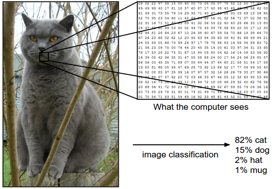

Challenges: Since this task of recognizing a visual concept (e.g. cat) is relatively trivial for human to perform, it is worth considering the challenges involved from the perspective of a CV algorithm. As we present list of challenges below.

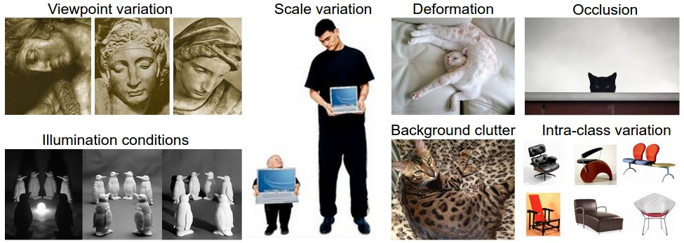
Viewpoint variation: A single instance of an object can be oriented in many ways with respect to the camera.
Scale variation: Visual classes often exhibit variation of their size (size in the real world, not only in terms of their extent in the image)
Deformation: Many objects of interest are not rigid bodies and can be deformed in extremes ways.
Occlusion: The objects of interest can be occluded. Sometimes only a small portion of an object (as little as few pixels) could be visible.
Illumination conditions: The effect of illumination are drastic on the pixel level.
Background clutter: The objects of interest may blend into their environment, making them hard to identify.
Intra-class variation: The classes of interest can be often be relatively broad, such as chair. Their are many different types of these objects, each with their own appearance.

A good image classification model must be invariant to the cross product of all these variations, while simultaneously retaining sensitivity to the inter-class variations.

Cross product of variations This refers to the combination of all possible variations (e.g. viewpoint, scale, deformation, occlusion, illumination, etc.) that can occur within a class. The term “cross production” here is metaphorical, inpsired by the mathematical concept of a Cartesian product, which generate all possible combinations of elements from multiple sets.
- Example: A chair might appear:
  - Rotate (viewpoint variation)
  - Partially hidden (occlusion)
  - Under bright sunlight (illumination)
  - While being non-rigid (deformation) The model must recognize it as a “chair” despite this complex combination of variations Invariance Requirement: The model must be invariant to these variations, meaning its prediction for a class should not change even when factors alter the object’s appearance.
Inter-class variation There are difference between distinct classes (e.g. chairs vs tables). A model must retain sensitivity to these differences to avoid confusing classes, even when they share superficial similarities.
- Example: A “stool” (class: chair) and a “small table” (class: table) might both appear at similar scales or under similar lighting. The model must distinguish them based on defining feature (e.g. height, presence of a backrest).
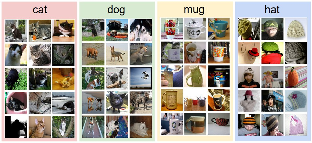
- Sensitivity Requirement: The model must preserver discriminate features that separate classes, even when intra-class variations (e.g. deformation in chairs) are extreme. Data-driven approach: How might we go about writing an algorithm that can classify images into distinct categories? Unlike writing an algorithm for, for example, sorting a list of numbers, it is not obvious how one might write an algorithm for identifying cats in images. Therefore, instead of trying to specify what every one of the categories of interest look like directly in code, the approach that we will take is not unlike one we would take with a child: we’re going to provide the computer with many examples of each class and then develop learning algorithms that look at these examples and learn about the visual appearance of each class. This approach is referred to as a data-driven approach, since it relies on first accumulating a training dataset of labeled images. Here is an example of what such a dataset might look like:

The image classification pipeline We’ve seen that the task in Image Classification is to taken an array of pixels that represents a single image and assign a label to it. Our complete pipeline can be formalized as follows: - Input: Our input consists of a set of N images, each labeled with one of K different classes. We refer to this data as the learning set. - Learning: Our task is to use the training set to learn what every one of the classes looks like. We refer to this step as training a classifier, or learning a model. - Evaluation: In the end, we evaluate the quality of the classifier by asking it to predict labels for a new set of images that it has never seen before. We will then compare the true labels of these images to the ones predicted by the classifier. Intuitively, we’re hoping that a lot of the predictions match up with the true answers (which we call the ground truth).

Nearest Neighbor Classifier

As our first approach, we will develop what we call a Nearest Neighbor Classifier. This classifier has nothing to do with Convolution Neural Networks and it is very rarely used in practice, but i will allow us to get an ideal about the basic approach to an image classification.

Example image classification dataset: CIFAR-10. CIFAR-10 datasetThis dataset consist of 10 classes (for example airplane, automobile, bird, etc). These 60,000 images are partitioned into a training set of 50,000 images and a test set of 10,000 images. In the image below we can see 10 random example images from each one of the 10 classes.

Left: Example images from the CIFAR-10 dataset. Right: first column shows a few test images and next to each we show the top 10 nearest neighbors in the training set according to pixel-wise difference.

Suppose now that we are given the CIFAR-10 training set of 50,000 images (5000 image for every one of the labels), and we wish to label the remaining 10,000. The nearest neighbor classifier will take a test image, compare it to every single one of the training images, and predict the label of the closest training image. In the image above and on the right we can see an example result of such a procedure for 10 example test images. Notice that in only about 3 of 10 examples of an image of the same class is retrieved, while in other 7 examples this is not the case. For example, in the 8th row the nearest training image to the horse head is a red car, presumably due to the strong black background. As a result, this image of a horse would in this case be mislabeled as a car.

One of the simplest possibilities is to compare the images pixel by pixel and add up all the differences. In other words, given two images and representing them as vectors \(I_1, I_2\), a reasonable choice for comparing them might be the L1 distance.

\[d_1(I_1, I_2)=\Sigma_p |I_1^p - I_2^p|\] Where the sum is taken over all pixels. Here is the procedure visualized:

![[nneg.jpeg]]

import numpy as numpy

class NearestNeighbor(object):
    def __init__(self):
        pass
    def train(self, X, y):
        """ X is N \times D where each row is an example. Y is 1-dimension of size N"""
        # the nearest neighbor classifier simpply remembers all the training data
        self.Xtr = X
        self.ytr = y
    def predict(self, X):
        """ X is N \times D where each row is an example we wish to predict label for"""
        num_test = X.shape[0]
        # lets make sure that the output type matches the input type
        Ypred = np.zeros(num_test, dtype = self.dtype)
        # loop over all test rows
        for i in range(num_test):
            # find the nearest training image to the i'th test image
            # using the L1 distance (sum of absolute value differences)
            distances = np.sum(np.abs(self.Xtr - X[i,:]), axis = 1)
            min_index = np.argmin(distances) # get the index with smallest distance
            Ypred[i] = self.ytr[min_index] # predict the label of the nearest example
        return Ypred

The choice of distance

k - Nearest Neighbor Classifier

The idea: instead of finding the single closest image in the training set, we will find the top k closest images, and have them vote on the label of the test image. In particular, when k=1, we recover the NN classifier. Intuitively, higher values of k have smoothing effect that makes the classifier more resistant to outliers:

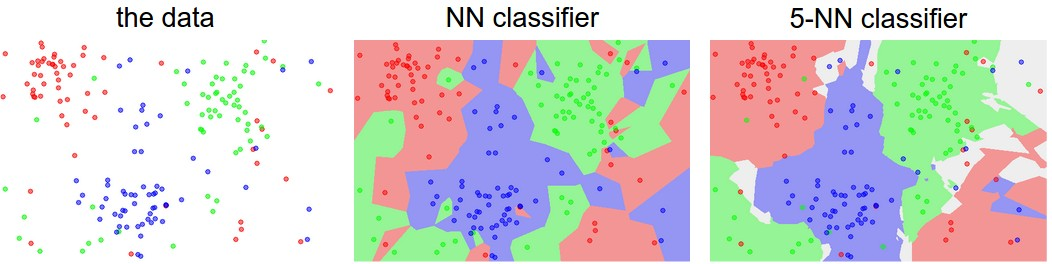
An example of the difference between Nearest Neighbor and a 5-Nearest Neighbor classifier, using 2-dimensional points and 3 classes (red, blue, green). The colored regions show the decision boundaries induced by the classifier with an L2 distance. The white regions show points that are ambiguously classified (i.e. class votes are tied for at least two classes). Notice that in the case of a NN classifier, outlier datapoints (e.g. green point in the middle of a cloud of blue points) create small islands of likely incorrect predictions, while the 5-NN classifier smooths over these irregularities, likely leading to better generalization on the test data (not shown). Also note that the gray regions in the 5-NN image are caused by ties in the votes among the nearest neighbors (e.g. 2 neighbors are red, next two neighbors are blue, last neighbor is green).

Validation sets for Hyperparameter tunning.

We saw that there are many different distance functions we could have used: L1 norm, L2. norm, there are many other choices we didn’t even consider (e.g. dot products). These choices are called hyperparameters nd they come up very often in the design of many ML algorithms that learn from data. It’s often not obvious what values/settings one should choose.

We might be tempted to suggest what we should try out many different values and see what work bests. That is a fine idea and that’s indeed what we will do, but this must be done very carefully. In particular, we cannot use the test set for the purpose of tweaking hyperparameters. Whenever we’re designing ML algorithms, we should think of the test set as a very precious resource that should ideally never be touched until one time at the very end. Otherwise, the very real danger is that we may tune our hyperparameters to work well on the test set, but if we were to deploy our model we could see a significantly reduced performance. in practice, we would say that we overfit to the test set. Another way of looking at it is that if we tune