2  Convex optimization

Author

Affiliation

Your name

Maybe your workplace?

3 Define

A convex optimization problem has the form

\[ \begin{aligned} & \underset{x}{\text{minimize}} & & f_0(x) \\ & \text{subject to} & & f_i(x) \le 0,\quad i=1,\dots,m,\\ & & & A x = b. \end{aligned} \]

• Variable: \(x\in\mathbb R^n\)
• Equality constraints: linear (\(A x = b\))
  
• Inequality constraints: \(f_1,\dots,f_m\) are convex functions

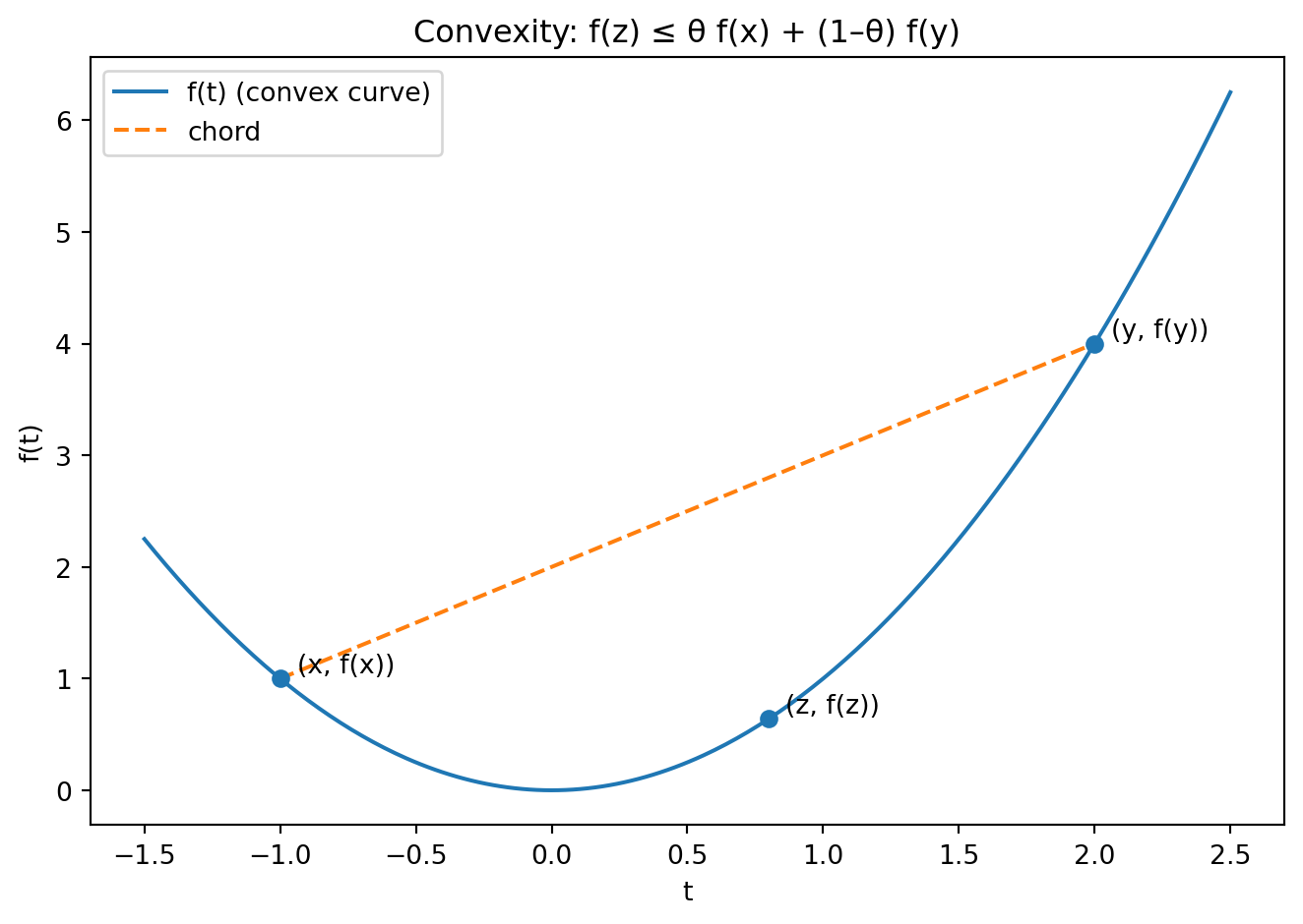
A function \(f\) is convex if, for all \(x,y\) and \(\theta\in[0,1]\), \[ f\bigl(\theta x+(1-\theta)y\bigr)\;\le\;\theta\,f(x)\;+\;(1-\theta)\,f(y), \] i.e. it has non-negative (upward) curvature.```mermaid

import numpy as np
import matplotlib.pyplot as plt

# convex function
f = lambda t: t**2

# pick x, y, theta
x, y, theta = -1.0, 2.0, 0.4
z = theta*x + (1-theta)*y

# sample for curve
t = np.linspace(x-0.5, y+0.5, 300)
plt.plot(t, f(t), label="f(t) (convex curve)")

# points
plt.scatter([x, y, z], [f(x), f(y), f(z)], zorder=5)
plt.text(x, f(x), "  (x, f(x))", va="bottom")
plt.text(y, f(y), "  (y, f(y))", va="bottom")
plt.text(z, f(z), "  (z, f(z))", va="bottom")

# chord
fx, fy = f(x), f(y)
chord = lambda t: fx + (fy-fx)/(y-x)*(t-x)
plt.plot([x, y], [fx, fy], '--', label="chord")

plt.legend()
plt.xlabel("t")
plt.ylabel("f(t)")
plt.title("Convexity: f(z) ≤ θ f(x) + (1–θ) f(y)")
plt.tight_layout()
plt.show()

When is an optimization problem hard to solve?

Classically, people thought:

Linear problems (zero curvature) are easy, and

Nonlinear problems (nonzero curvature) are hard.

However, this view is too simplistic. The key distinction is actually convexity:

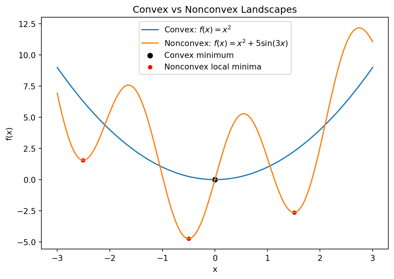
Convex problems (nonnegative curvature) can be solved reliably in polynomial time using interior-point methods, gradient-based schemes with global convergence guarantees, and other efficient algorithms. The feasible set and objective have no ‘valleys’ that trap algorithms in suboptimal points.

Nonconvex problems (regions of negative curvature) are generally NP-hard. They can exhibit multiple local minima, saddle points, and complex landscape features, so finding the global minimum is computationally intractable in the worst case (unless P=NP).

Thus, the presence of negative curvature (nonconvexity) — not merely ‘nonlinearity’ — is what makes an optimization problem hard to solve.

import numpy as np
import matplotlib.pyplot as plt

# Define convex and nonconvex functions
convex = lambda x: x**2
nonconvex = lambda x: x**2 + 5*np.sin(3*x)

# Domain
x = np.linspace(-3, 3, 500)

# Plot both functions
plt.figure()
plt.plot(x, convex(x), label='Convex: $f(x)=x^2$')
plt.plot(x, nonconvex(x), label='Nonconvex: $f(x)=x^2+5\sin(3x)$')

# Mark minima
# For convex, minimum at x=0
plt.scatter(0, convex(0), color='black', label='Convex minimum')
# For nonconvex, approximate local minima
d = nonconvex(x)
idx = (np.diff(np.sign(np.diff(d))) > 0).nonzero()[0] + 1
plt.scatter(x[idx], d[idx], color='red', s=20, label='Nonconvex local minima')

plt.title('Convex vs Nonconvex Landscapes')
plt.xlabel('x')
plt.ylabel('f(x)')
plt.legend()
plt.tight_layout()

negative curvature (nonconvexity) — not merely ‘nonlinearity’ — is what makes an optimization problem hard to solve.